Vibration Analysis for Fault Diagnosis of Cycloidal Gearbox Using Wavelet Transform

Nomenclature FFT Fast Fourier Transform WT Wavelet Transform X(t) Signal to be analyzed, in 1d }0(t) Mother wavelet j Scale of Wavelet Transform k Position in time shift Share and save: This article appeared in the September 2026 issue. Read PDF [advertisement] Dx(j, k) Discrete wavelet transform coefficient H Hurst or self-similar parameter h Hölder exponent g(q) The scaling function of Multifractal analysis c1, c2 Cumulants, to quantify the strength of the multifractality. If c2=0, the process is monofractal; otherwise, multifractal. Sq(j) Structure function: it represents the qth moment of the wavelet leaders at each scale j D(h) Multifractal spectrum OR Singularity spectrum L(j, k) Wavelet leaders at scale j and position k q Moment N Number of wavelet leaders available at scale 2j [advertisement] CPM Cycle per minute

Introduction

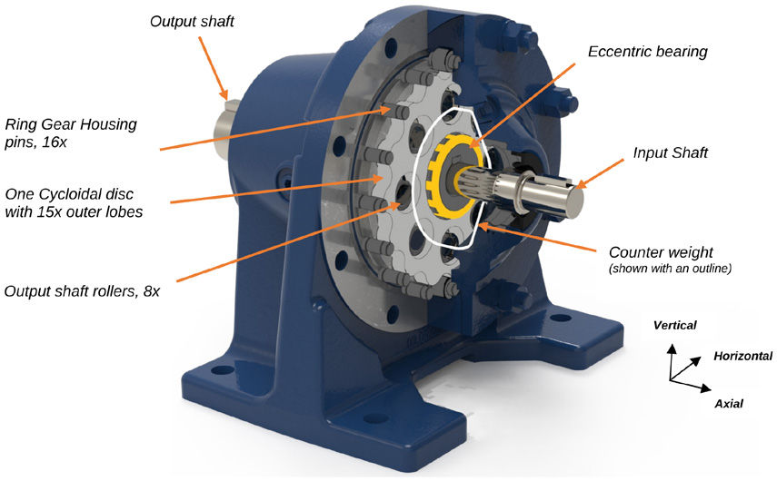
For years, the cycloidal reducer (Figure 1) has proven its performance in a variety of applications, from robotics to wastewater treatment. Along with involute gearing, the cycloidal mechanism has its place in the mechanical power transmission world. It is well known for its high torque density, high integer ratio per stage, and shock load handling capabilities. Its poke-yoke assembly refrains from introducing any errors during assembly and allows the unit to operate with low maintenance. Despite these advantages, the reducer may have a variable angular speed at its output shaft, in large part due to manufacturing imperfections. A constant transmission ratio during gear meshing can be attained with involute gearing by following standardized methods established in the gearing industry (Ref. 1). Considering the manufacturing deviations and loading conditions, one could optimize the macro and micro geometries of the involute gearing and get a fairly controlled transmission error. In the case of cycloidal gearing, however, the same may not hold. The steadiness of the ratio, or the output shaft's angular velocity, will vary with the cycloidal gearbox manufacturer. Small dimensional deviations in rotating components, such as the cycloidal disc and rollers, will influence the variations in the output shaft rotation. The torque load on the output shaft also induces the variation. Such scenarios have the potential to negatively influence traditional vibration-based fault diagnosis methods.

Vibration analysis has long been sought for condition monitoring and fault diagnosis of rotating equipment or machinery. Conventional methods utilize analyzing the time spectrum and frequency spectrum with fast Fourier transform (FFT), or in many instances both. The raw vibration data or signal recorded by the accelerometer generates the time spectrum with no additional signal processing. The time waveform is useful in identifying modulation and pulses in the signal. When frequencies of the rotary components in the gearbox are known, the same signal can be processed with FFT to obtain the frequency spectrum and then locate high-energy generating or out-of-sync components. The wide acceptance of FFT hinges on the assumption that the processed signal is stationary, meaning all the frequencies in the signal exist in all instances, and they do not vary with time. The stationary signal, hence, does not depend on the data sampling period or recording instances (Ref. 2). This assumption fails when the angular speed of the gearbox shafts fluctuates due to transmission error and load fluctuations, and the signal becomes non-stationary, or time-dependent.

It is worth mentioning that the involute and cycloidal gearing differ in their primary failure modes. In involute gearing, the common failure is tooth breakage. In (epi)cycloidal gearing, as the cycloidal disc lobes (equivalent to the gear teeth) experience less shear force with a much higher contact ratio, they tend to break less. The common maintenance issues for a cycloidal gearbox would be a worn-out cycloidal disc, eccentric bearing, or damage to the ring gear housing pins. Therefore, the conventional way of fault diagnosis may not effectively capture such subtle changes.

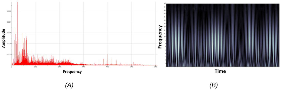
The FFT-processed signal has no time (or phase) related information in it. The nonstationary signal raises a need to know when an event has taken place on a timeline, along with its appearance on the frequency scale. Analyzing the separate graphs of time and frequency side-by-side may not be intuitive. If one tries to put time and frequency on one graph, it is well known that Heisenberg’s Uncertainty Principle would allow resolution of the signal for one of the components (time or frequency), but not both. To overcome this limitation, various time-frequency analysis methods were developed by sacrificing some resolution in both components. Among those methods are the short-time Fourier transform, Wigner-Ville Distribution, and wavelet transform (WT) (Ref. 3). Typical graphs of FFT and WT are shown in Figure 2 for comparison purposes. Each line in the FFT graph represents a frequency with a certain amplitude, whereas in the WT Scalogram, the brightness of each band signifies the strength of the frequency component in a specific frequency range seen on the Y-axis, at a certain time.

Since its introduction in 1982, the WT method has gained more interest in vibration measurements (Ref. 4). The French word wavelet means a “small wave.” In WT signal analysis, a wavelet function (or a predetermined signal) is blended with the signal to be analyzed using convolution to extract necessary information. This information about the signal could capture singular events that the Fourier Transform treats as anomalies and ignores. For instance, an event of tooth loss of the involute gear appears as a singularity in the time spectrum, but it is hard to capture in the frequency spectrum. In the frequency spectrum, it shows up in sidebands to the gear mesh frequency. The sideband, however, truly attributes to the frequency or amplitude modulation and not necessarily to the defect. In other instances, the singularities are buried in the vibration data and impossible to identify in any of the above-mentioned spectra. These events or singularities are also defined as fractal features. The term fractal was coined to denote geometries and patterns that could not be defined with Euclidean geometry (Ref. 5). The simplest way to comprehend fractals is with Taylor series. A function f(t) is approximated around a certain time t_i as below:

(1)

where p_i is a non-integer number quantifying the local singularity of the function f(t) at t=t_i, with a_h coefficient. Here, the non-integer exponent is referred to as a singularity exponent, and due to this exponent, the function approximates the singular behavior, which would be ignored when an integer exponent is used.

Another important aspect of WT is that it generates coefficients that are associated with the singularities embedded in the signal. The signal could be a monofractal, i.e., having a single coefficient to represent all singularities, or multifractal. The popular applications of multifractal analysis are modeling turbulent flow of gases, stock markets, image processing, and filtering heartbeat signals to display on an electrocardiogram or ECG (Refs. 6,7,8).

In this paper, WT will be used to detect fractals embedded in the vibration data to demonstrate its benefit in distinguishing a cycloidal reducer fault, which otherwise would go undetected.

Literature Review

Multiple research papers have demonstrated the use of WT-based multifractal analysis to diagnose faults in rotary machinery. In the case of ball bearings, when multiple faults with different diameters and depths are present on both inner and outer races, the time/ frequency spectrum could distinguish a very few of them (Ref. 9). The paper focuses on comparing a variety of induced faults in ball bearings using the WT modulus maxima method. It shows that different fault conditions would carry the fault information in the form of a distribution of singularities. The multifractal spectrum and scaling exponents can be clearly distinguished.

One interesting application of multifractal analysis is in material testing. To identify progression of the failure in a structural composite material, the multifractal spectrum and fractal leaders could be deployed to observe nonstationary changes in the vibration signal (Ref. 10). In this experiment, vibratory signals generated during a composite bending test were recorded. The test progressed in three stages until the failure of the specimen. Each stage generated fractals that were plotted on a singularity spectrum to differentiate from each other. The holder coefficients increase with increased bending and thus would help to indicate the initial or final stage of the failure.

The gear fault analyses were performed on spur gear pairs to demonstrate the use of WT (Refs. 11,12). For these analyses, multiple gear pairs showing different stages of the bending fatigue failure progression were mounted on test rigs, and vibration samples were analyzed. For instance, Ref. 11 shows how the distribution of the scaling exponents changes from a healthy gear with no cracks to the fatigue crack magnitude of 15 percent, 50 percent, and 75 percent of the gear tooth root, and subsequently relates to tooth loss. Such progression of the failure would not be easy to distinguish by observing FFT and the power spectral density graphs. These studies deploy fault detection algorithms to perform gear diagnostics. Along with gear fault diagnosis, the WT method has also been used to simulate gear misalignment due to assembly error and variation in clearance (Ref. 13). These faults, when recorded in separate tests and plotted on the multifractal spectra, show differences in the singularity distributions. Singularity subsets, called cumulants, were fed to machine learning methods, such as neural network (NN), K-NN, and support vector machine (SVM), to classify the gearbox state.

In the case of Cycloidal gearbox fault diagnosis, the benefits of the WT are demonstrated by comparing the vibration data gathered from the faulty and non-faulty Cyclo reducers (Ref. 14). The paper argues that the conventional FFT falls short in distinguishing these two reducers. To create a fault in the gearbox, two rotary components, in this case ring gear housing pins, were removed (refer to Figure 1). Plots of multifractal spectra and two-cumulant dispersions show clear separations of faulty and non-faulty data. The removal of the components may represent an assembly error. However, it does not specifically depict flaws such as component fracture, wear, or manufacturing error (clearance due to inadequate tolerance). Another paper on cycloidal fault diagnosis uses actual worn-out parts, including the disc and eccentric bearing, but only considers FFT in vibration analysis (Ref. 15). The current paper intends to extend the aforementioned analyses and perform WT multifractal analysis on a simulated worn-out cycloidal disc.

The objective of this paper is to diagnose a cycloidal gearbox by utilizing discrete wavelet transform analysis and compare the findings with FFT.

Wavelet Transform Multifractal Analysis

A signal X(t) in 1d can be decomposed with WT by using a known function or mother wavelet, }₀(t), into scales that correspond to frequencies. When plotted against the time shift on the X-axis, a time-frequency graph can be achieved (refer to Figure 2B). In this work, discrete wavelet transform (DWT) is utilized as it is computationally more efficient than continuous wavelet transform (CWT). The DWT coefficients are defined as:

(2)

The coefficients are then further used to derive Wavelet Leaders L(j, k) in the multifractal analysis, as they are the largest coefficients in a certain time neighborhood (local supremum) and possess significant qualities to construct a multifractal formalism (Ref. 16). This can be elaborated by defining dyadic intervals:

(3)

So, the wavelet leaders are defined as:

(4)

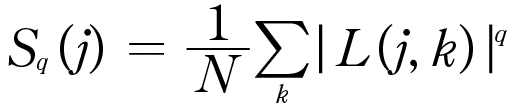
Wavelet leaders multifractal formalism (WLMF) in plotting the multifractal spectrum and log cumulants. The structure function derived from the wavelet leaders is defined as:

(5)

The scaling function g(q)

(6)

Here, when the cumulant c₂=0, the signal is monofractal and has the same scaling in entire data. when c₂≠0, the signal is multifractal. The structure function follows a power-law scaling over scales

(7)

The local regularities are described by Hölder exponent h, and the multifractal spectrum D(h) represents the distribution of singularities in the signal.

(8)

Experimentation with Cycloidal Gearbox

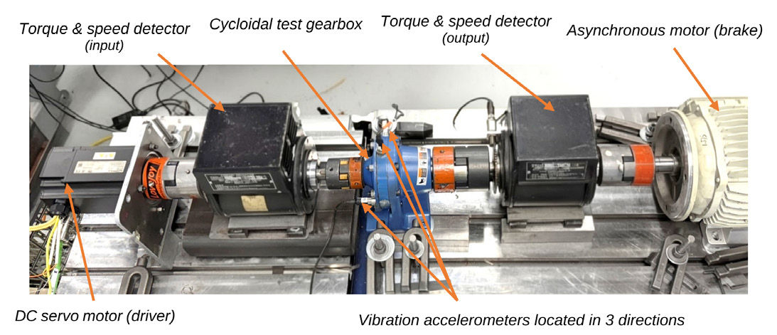
The vibration measurements were carried out on a test stand shown in Figure 3. A Sumitomo cycloidal gearbox of a 15.00:1 ratio was selected for the experiment. CNH-609 gearbox was specifically chosen as it consists of one cycloidal disc (Ref. 17). In lieu of the second disc, which exists in a typical cycloidal reducer, this gearbox design uses a counterweight to achieve dynamic balancing (refer to Figure 1). The one-disc mechanism simplifies the analysis and allows focusing on certain frequencies. In the setup, the gearbox was driven by a DC Servo motor with an encoder feedback loop to provide a consistent speed of 1,800 rpm (30 Hz). The DC motor’s torque capacity was 2.39 Nm. The output shaft of the gearbox was connected to the asynchronous motor that acted as a brake. The torque and speed were measured using torque meters and encoders, respectively, for both input and output shafts. Three vibration sensors (sensitivity 87 mV/g at 6000 CPM) were mounted on the gearbox to collect tri-axial vibration data. All measurements were recorded using the National Instruments Data Acquisition (NI DAQ) system at a sample rate of 12.8 kHz for vibration and 10 kHz for torque measurements. For the input shaft spinning at 30 Hz, the DAQ system would generate 426 and 333 data points for vibration and torque, respectively, in one revolution of the shaft.

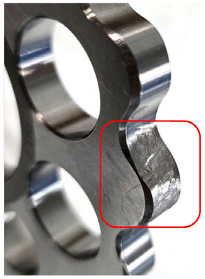
The gearbox was assembled with the standard lubricant using an NGLI 00 grade grease, with a predefined quantity. To confirm that all test iterations were performed at a steady temperature, the test stand was placed in a climate-controlled room with an ambient temperature of 21°C. Two temperature probes were placed to monitor the reduction housing or ‘ring gear’ housing of the gearbox. The load on the reducer output shaft was varied from 0 Nm to 15 Nm during the experimentation. The gearbox was tested for a healthy condition, meaning it had no induced errors. Then it was tested for a worn-out cycloidal disc or damaged condition by swapping out the normal disc with the one seen in Figure 4. Other than the disc, the use of the same parts in both conditions ensured that there were no other changes to influence the vibration data. It is important to highlight the fact that the induced change in the ‘damaged’ condition is relatively small. The goal of the testing was to gather vibration data and analyze it with FFT and multifractal analyses.

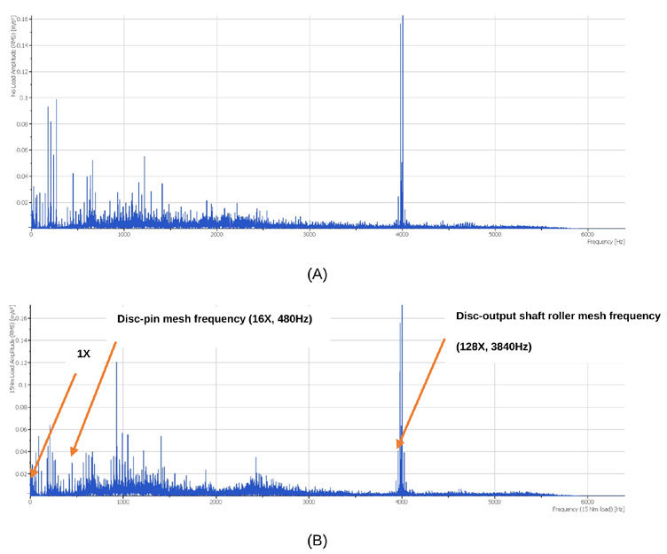
Referring to Figure 1, the cycloidal reducer utilized for the experiment has a cycloidal disc with 15 lobes. These lobes engage with 16 ring gear housing pins when the eccentric bearing sways the disc with its eccentricity. The ‘engaged’ disc (with pins) then generates a rotary motion while it is swaying and forces the output shaft to spin with the reduced speed in the opposite direction. The connection between the disc and the output shaft is achieved by engaging 8 output rollers within the 8 holes of the disc. This information helps to determine the mesh frequencies. The disc-pin mesh frequency is 16x order. The disc-output shaft roller mesh frequency is 16x8 = 128x order.

Results and Discussion

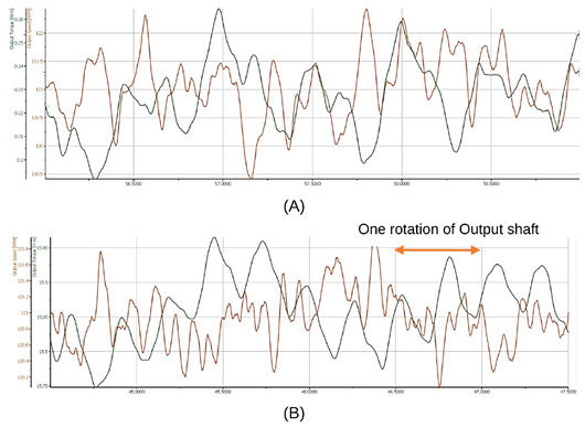
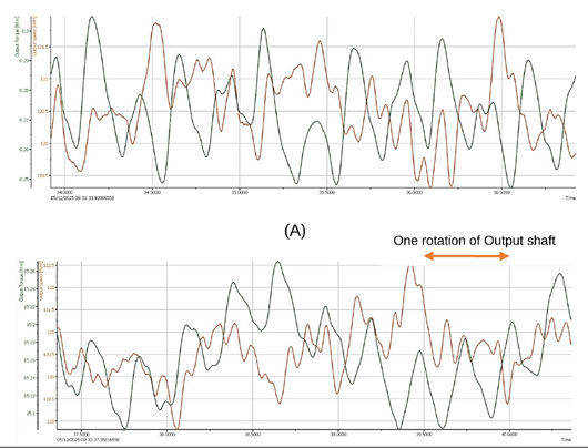
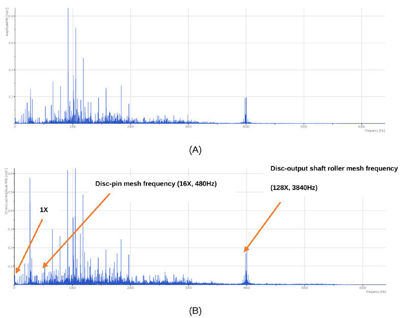
Figure 5 and Figure 7 show the torque and speed curves for healthy and damaged gearbox conditions. Each condition has 0 Nm and 15 Nm loads. Both torque and speed curves depict the steadiness of the power (proportional to the product of torque and speed) flowing through the system by generally showing opposite trends to each other. The variation in those curves over the period of three seconds confirms the randomness of the signal, hence categorizing it as a nonstationary signal. The FFT would assume the same signal as stationary, i.e., the signal not varying with time. This assumption ignores the local irregularity or fractals, and hence potentially any evidence of the fault existence. When the signal of one second period was FFT processed and plotted against the RMS amplitude in m/s² (refer to Figures 6 and 8), the aforementioned cycloidal mesh frequencies can be observed.

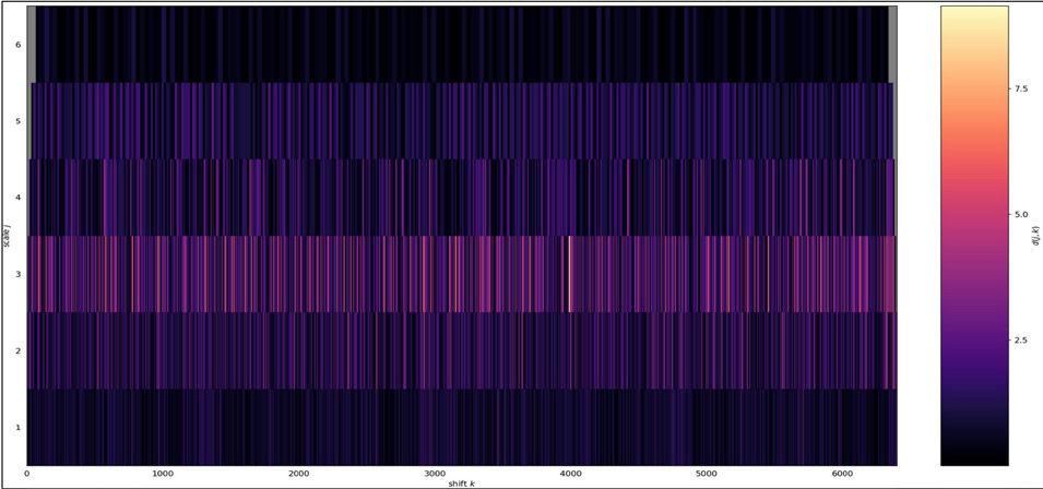
A typical way to diagnose any faulty machine using vibration is to compare its pre- and post-incident data, which means comparing the healthy (Figure 6) and the damaged reducer (Figure 8) graphs. However, apart from observing the higher amplitudes across the spectrum, it was incomprehensible to establish any relation with the fault by utilizing known frequencies (highlighted in graphs). Even at 16× order (disc-pin mesh frequency), where the fault was induced, no noticeable relative data change was observed. The same time period (one second) vibration data was then analyzed with WT, by plotting the Scalogram shown in Figure 9. As discussed in the “Introduction” section, the Scalogram or “Frequency vs Time” graph generally reveals the dominant frequencies at a time instant inside the non-stationary signal. Figure 9 shows a burst in localized activities, confirming the existence of mono- or multifractality in the signal generated by the damaged gearbox. Equations 4–8 were used to perform Multifractal analysis to extract wavelet coefficients that built the Scalogram, to derive the multifractal spectrum. The multifractal spectrum is plotted in Figure 10 for all three axes of vibrations: vertical, horizontal, and axial. The axis diagram, referred to in Figure 1, has the reducer shaft axis aligned with the vibration axial direction, and the remaining axes are in the radial direction of the cycloidal disc.

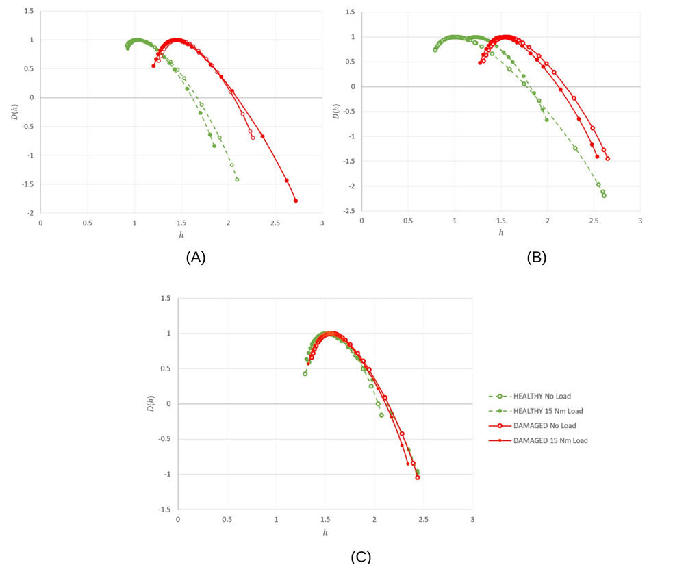
Each graph in Figure 10 consists of four curves showing different operating conditions of the gearbox: a healthy reducer with no load, a healthy reducer with 15 Nm load, a damaged reducer with no load, and a damaged reducer with 15 Nm load. Based on their positioning on the graph, the curves can visibly be sorted into healthy and damaged groups (green color and red color, respectively) in Figure 10(A) and Figure 10(B). The damaged gearbox’s curves are shifted towards the right side of the multifractal spectrum, making them separated from the healthy ones. It can be argued that the main cause of this distinction was the induced damage on the cycloidal disc. The worn-out surface on the disc generated singularities affecting the wavelet coefficients, subsequently creating a deviation in the multifractal spectrum in radial directions. The axial axis graph, Figure 10(C), does not show similar shifting, as the worn-out lobe of the disc would not have energy change in this direction. The loading conditions, 0 Nm and 15 Nm, do not noticeably influence the shifting in all three graphs.

Conclusion

The paper compares results of the two tests conducted on the same gearbox. The only difference between the two test setups was the condition of Cycloidal disc, depicting ‘healthy’ in one and ‘faulty’ in another. The multifractal spectrum clearly distinguished the vibration data with respect to their conditions, which Fast Fourier Transform graphs could not. This paper argues that the wavelet transform based multifractal analysis approach makes the Cycloidal gearbox diagnosis less ambiguous compared to FFT. This is mainly because the collected vibration signals were time dependent and the singularities in the signal cannot be captured using FFT. The multifractal spectra also showed that the load on the gearbox output shaft does not significantly influence the curve shifting or the Hölder coefficient. For the future work, it is worth exploring the ‘worn-out’ effect of other Cycloidal gearbox components, such ring gear pins, output rollers, on the multifractal spectrum and establish the changes to be utilized in fault diagnostics.

References

1. ANSI/AGMA 6002-D20, Design guide for vehicle spur and helical gears, 2020, AGMA.

2. R. B. Randall, Frequency analysis, 3rd ed. Naerum: Brüel & Kjaer, 1987.

3. K. G.-H. Svend Gade, “Technical Review: Non-stationary Signal Analysis using Wavelet Transform, Short-time Fourier Transform and Winger-Ville Distribution,” Bruel & Kjaer, 1996.

4. J. Morlet, G. Arens, E. Fourgeau, and D. Giard, “Wave propagation and sampling theory; Part II, Sampling theory and complex waves,” Geophysics, Vol. 47, No. 2, pp. 222–236, Feb. 1982, doi: 10.1190/1.1441329.

5. B. B. Mandelbrot, The Fractal Geometry of Nature. New York: W.H. Freeman and Company, 1977.

6. C. Meneveau and K. R. Sreenivasan, “Simple multifractal cascade model for fully developed turbulence,” Phys Rev Lett, Vol. 59, pp. 1424–1427, 1987.

7. D. Lin and R. Hughson, “Modeling Heart Rate Variability in Healthy Humans: A Turbulence Analogy,” Phys Rev Lett, Vol. 86, pp. 1650–1653, May 2001, doi: 10.17877/DE290R-16101.

8. H. Wendt, S. G. Roux, S. Jaffard, and P. Abry, “Wavelet leaders and bootstrap for multifractal analysis of images,” Signal Processing, Vol. 89, No. 6, pp. 1100–1114, 2009, [Online]. Available: http://dx.doi.org/10.1016/j.sigpro.2008.12.015

9. W. Du, J. Tao, Y. Li, and C. Liu, “Wavelet leaders multifractal features based fault diagnosis of rotating mechanism,” Mech Syst Signal Process, Vol. 43, No. 1, pp. 57–75, 2014, doi: https://doi.org/10.1016/j.ymssp.2013.09.003.

10. T. Figlus and M. Kozioł, “Application of the Multifractal Spectrum to the Analysis of Vibration Signals Generated During Testing of Selected Composite Materials,” Advances in Science and Technology Research Journal, Vol. 18, No. 7, pp. 123–137, 2024, doi: 10.12913/22998624/192616.

11. W. J. Staszewski and G. R. Tomlinson, “Application of the wavelet transform to fault detection in a spur gear,” Mech Syst Signal Process, Vol. 8, No. 3, pp. 289–307, May 1994, doi: 10.1006/mssp.1994.1022.

12. S. J. Loutridis, “Self-similarity in vibration time series: Application to gear fault diagnostics,” J Vib Acoust, Vol. 130, No. 3, 2008.

13. A. Puchalski and I. Komorska, “Data-driven monitoring of the gearbox using multifractal analysis and machine learning methods,” MATEC Web Conf., Vol. 252, 2019.

14. Komorska, K. Olejarczyk, A. Puchalski, M. Wiklo, and Z. Wolczyski, “Fault Diagnosing of Cycloidal Gear Reducer Using Statistical Features of Vibration Signal and Multifractal Spectra,” Sensors, Vol. 23, No. 3, 2023, doi: 10.3390/s23031645.

15. V. Cochran and T. Bobak, “A methodology for identifying defective cycloidal reduction components using vibration analysis and techniques,” in American Gear Manufacturers Association—American Gear Manufacturers Association Fall Technical Meeting 2008, San Antonio, TX, United States, 2008, pp. 8–32.

16. H. Wendt, “Contributions of Wavelet Leaders and Bootstrap to Multifractal Analysis: Images, Estimation Performance, Dependence Structure and Vanishing Moments. Confidence Intervals and Hypothesis Tests,” May 2008.

17. Sumitomo, “Cyclo Reducer Catalog,” 2025.